Introducing Aplot

With the release of version 2.36, Simply Fortran now includes Aplot, a library for creating simple, two-dimensional plots and charts directly from Fortran.  The programming interface provided is designed to be straightforward, and the library is available on Windows, macOS, and GNU/Linux.  This short article will walk through creating a non-trivial plot quickly with Aplot.

For this example, we’ll attempt to plot 1000 random, uniformly distributed numbers along with a running mean as the sample size grows. The plot will therefore include scatter elements and a line, both with a significant amount of data.

In order to use Aplot, the aplot module must be employed in a given procedure:

use aplot

On Windows and macOS, this module will be seamlessly included. On GNU/Linux, Simply Fortran might show the module as unavailable until you click Build Project for the first time. There are no other steps to take; Simply Fortran will automatically detect this module’s inclusion and configure the compiler to link to the aplot library.

To generate our data set, we’ll need to populate some arrays accordingly. The code below should be sufficient:

    real, dimension(1000)::x, rand_y, mean_y
    integer::i
    
    call RANDOM_NUMBER(rand_y)
    
    do i = 1, 1000
        x(i) = real(i)
        mean_y(i) = sum(rand_y(1:i))/x(i)
    end do

The above code creates three arrays. Our X-axis data will just be the sample count, though we have to use a REAL variable with Aplot. The random data is created with a single call to RANDOM_NUMBER, which populates the entire rand_y array in one call.

The x array is manually populated inside the loop along with the calculation of a running mean in the mean_y array. This code generates two datasets that we need to plot.

In order to create a plot, we need to define a plot variable, which is of the aplot_t type:

type(aplot_t)::plot

This variable is used for defining all aspects of our plot at eventually displaying it. Before we can use it, though, we must initialize it:

    plot = initialize_plot()

Once initialized, we can define some aspects of our plot:

    call set_title(plot, "Uniform Random Numbers")
    call set_xlabel(plot, "Sample")
    call set_ylabel(plot, "Value")
    call set_yscale(plot, 0.0, 1.2)

Most calls above are straightforward, and each requires our plot variable as its first argument. The final call, though, to set_yscale might not be as obvious as setting titles and labels. By default, Aplot autoscales both axes. In this case, though, we know the data on the y-axis will fall between 0 and 1. In order to provide a little extra space, we’ll expand the plot slightly so that the y-axis varies from 0 to 1.2.

The next step is to configure each dataset for the plot. To add data, we must pass an X and Y array to the add_dataset subroutine:

    call add_dataset(plot, x, rand_y)

Once we’ve provided the first dataset to the plot, we can assign some attributes to the series:

    call set_seriestype(plot, 0, APLOT_STYLE_PIXEL)
    call set_serieslabel(plot, 0, "Random Number")

The call to set_seriestype configures the style of the series when drawn. The index of zero is passed because Aplot uses 0-indexing for its series identification. In this case, since we’ll be showing 1000 points, we’ve asked for it to be drawn as a scatter plot using single pixels; the user can also use larger dots, lines, or bars to represent a series. The second call to set_serieslabel provides a label for this series in the legend.

Our second dataset, the running average, can be configured similarly:

    call add_dataset(plot, x, mean_y)
    call set_seriestype(plot, 1, APLOT_STYLE_LINE)
    call set_serieslabel(plot, 1, "Running Mean")

Our plot is now entirely ready to display. The final step is to call:

    call display_plot(plot)

which opens a window displaying the complete plot.

The final coding step is to clean up our plot after the user closes it. While not necessarily important in a standalone program, a subroutine that generates plots should always perform final cleanup before exiting. The simple code is:

    call destroy_plot(plot)

After this call, all memory associated with the plot is released, and the program can continue normally.

The code here should compile in Simply Fortran 2.36 without issue, generating the following on GNU/Linux:

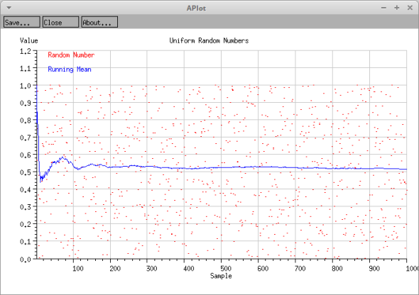
While the plot might look slightly different on macOS or Windows, it should still resemble the above chart.  The plot shows the running average, in blue, converging towards 0.5 as more samples are  considered.

Hopefully the above helps users get started with Aplot.  The interface is designed for quickly and easily adding plots to Fortran.   Any questions about how it works can always be posted on our forums, where either Approximatrix or another user will happily help  out.

The complete code for this example is below:

program ranmean
use aplot
implicit none

    type(aplot_t)::plot
    
    real, dimension(1000)::x, rand_y, mean_y
    integer::i
    
    call RANDOM_NUMBER(rand_y)
    
    do i = 1, 1000
        x(i) = real(i)
        mean_y(i) = sum(rand_y(1:i))/x(i)
    end do
    
    plot = initialize_plot()
    call set_title(plot, "Uniform Random Numbers")
    call set_xlabel(plot, "Sample")
    call set_ylabel(plot, "Value")
    call set_yscale(plot, 0.0, 1.2)
    
    call add_dataset(plot, x, rand_y)
    call set_seriestype(plot, 0, APLOT_STYLE_PIXEL)
    call set_serieslabel(plot, 0, "Random Number")
    
    call add_dataset(plot, x, mean_y)
    call set_seriestype(plot, 1, APLOT_STYLE_LINE)
    call set_serieslabel(plot, 1, "Running Mean")
    
    call display_plot(plot)
    
    call destroy_plot(plot)

end program ranmean